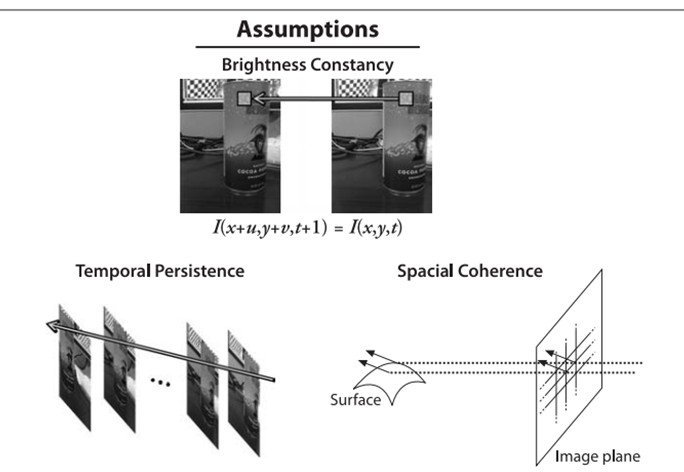
This is the time that I learn the Optical Flow,and the improtant algorithm-Lucas Kanade method.

Quote from http://en.wikipedia.org/wiki/Lucas%E2%80%93Kanade_Optical_Flow_Method

and “learning openCV”

In computer vision, this method is a two-frame differential method for optical flow estimateion developed by Bruce D.Lucas and Takeo Kanade. And ti introduces an additional term to the optical flow by assuming the flow to be constant in local neighbourhood around the central pixel under consideration at any given time.

The basic idea of the LK algorithm rests on three assumptions:

1, Brightness constancy

2, Temporal persistence or small movements

3, Spatial coherence

Figure 1 assuptions behind Lucas-Kanade optical flow

And for those assumptions we get those equals:

1,brightness constancy,

and it means that our tracked pixel intensity exhibits no change over time,

like

2, temporal persistence & spatial coherence,

 ,and in this partial differentiation,Ix is the spatial derivative across the first image, It is the derivative between images over time, and v is the velocity we are looking for. Then we arrive at the simple equation for optical flow velocity in the simple 1-dimosional case:

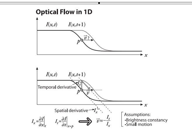
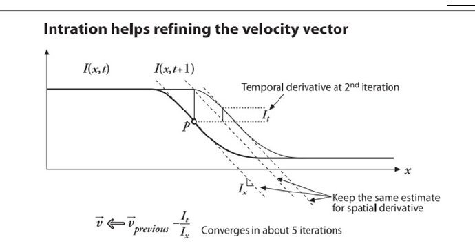
Figure 2 Lucas-Kanade optical flow in one dimension

While in the real world, our assumptions are not probably quite ture.for the reason that image brightness is not really stable, and time steps are often not exact. There we get the “intration” that helps refining the velocity vector.

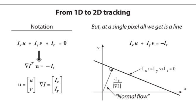
Figure 3 iterating to refine the optical flow solution(Newton’s method)

Now that we have seen the 1-dimension solution, then we generalize it to images in 2-dimensions.

In principle, we just want to add in the y coordinate, and slightly changing notation. We’ll call the y component of velocity v and the x component of velocity u; then we get :

 and figure 4 presents the mathematical and geometric details

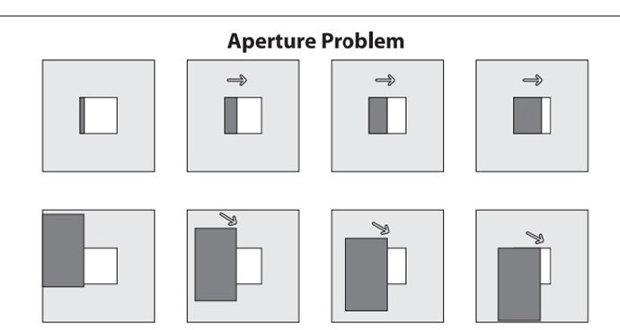
Figure 4 2-dimensional optical flow at a sigle pixel

And then another problem works out for aperture problem. When motion is detected with a small aperture, we often see only an edge,not a corner. But an edge alone is insuffcient to determine exactly how the entire is moving. This reason for figure 5

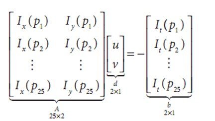
Figure 5 aperture problem: through the aperture window(upper row) we seen an edge moving to the right but cannot detect the downward part of the motion(lower row)

For this problem we turn to the last optical flow assumption. If a local patch of pixels moves coherently, then we can easily solve for the motion of the central pixel by using the surrounding pixels to set up a system of equations. We set up a least squares minimization of equation, and get the result. For instance, there a window  by 5-by-5 of brightness values around the curent pixel to compute its motion. We can then set up 25 equations as fallows :

We then use least squares minimiztion of this equation to solve for overconstrained system,whereby min||Ad-b||^2 is solved in standard form as:

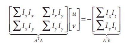
From this relation we present the detail yields for obtaining our u and v motion components

And then solution to this equation is

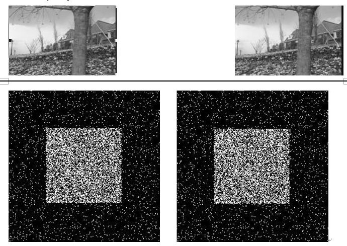
And the last when (A^TA) is invertible, this equation will be solved. And this matrix has full rank, which occures when it has two large eigenvectors. And the problem will ties the dicussion of the Harris corner detector.

In fact Lucas-Kanade method are not efficent for we need large window which too often breaks the coherent motion assupion to catch large mothions.There we use image pyramid to circumevent this problem: we can track first over larger spatial scacles using an image pyramid and then refine the initial motion velociy assumptions by working our way down the image pyramid until we arrive at the raw image pixels

There I got the code from “learning openCV”

Here are my test pictuer

And the result is

D:>lucas_kanade.exe 1.jpg 2.jpg 4.jpg

This is code here

// Pyramid L-K optical flow example

//

#include <cv.h>

#include <cxcore.h>

#include <highgui.h>

const int MAX_CORNERS = 500;

int main(int argc, char** argv)

    printf("Got it ");

    CvPoint p0 = cvPoint(cvRound( cornersA[i].x ),cvRound( cornersA[i].y ));

    CvPoint p1 = cvPoint(cvRound( cornersB[i].x ),cvRound( cornersB[i].y ));

    cvLine( imgC, p0, p1, CV_RGB(255,0,0),2 );

  }

  cvNamedWindow("ImageA",0);

  cvNamedWindow("ImageB",0);

  cvNamedWindow("LKpyr_OpticalFlow",0);

  cvShowImage("ImageA",imgA);

  cvShowImage("ImageB",imgB);

  cvShowImage("LKpyr_OpticalFlow",imgC);

  cvWaitKey(0);

  return 0;

}